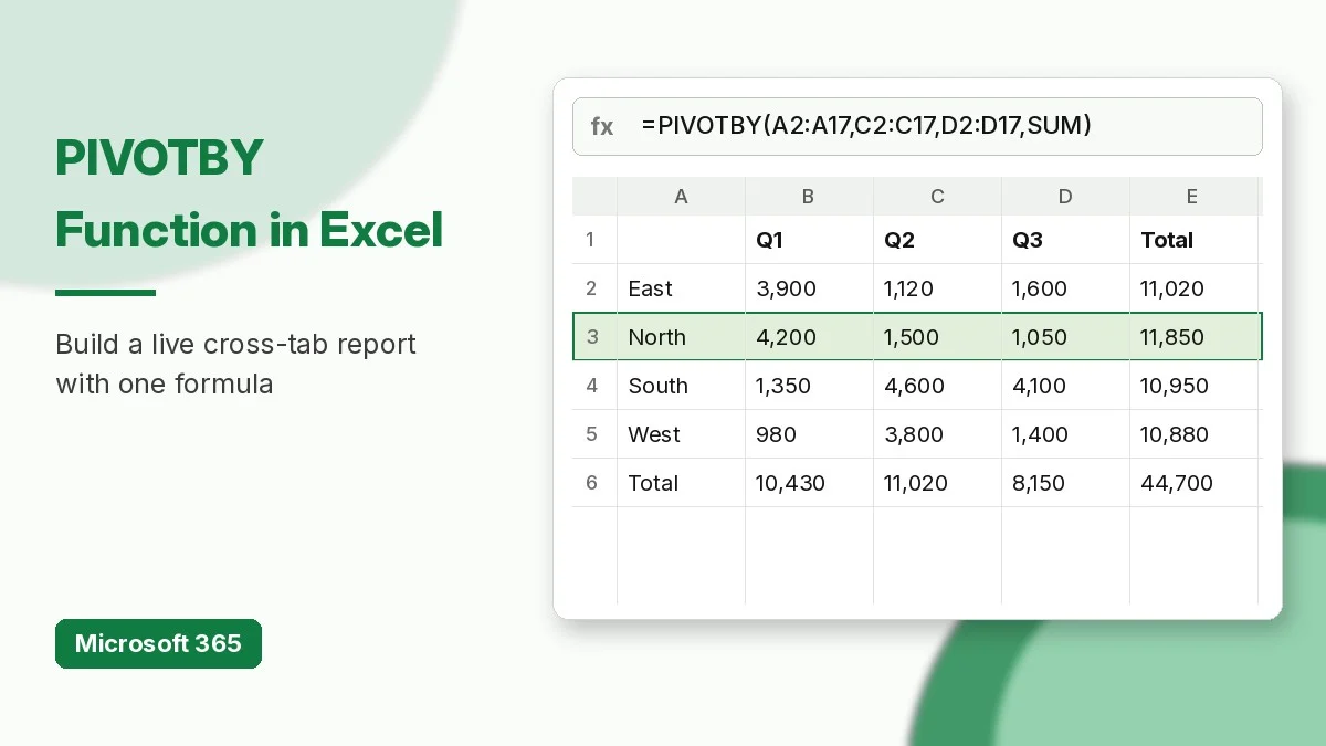
The PIVOTBY function in Excel builds a two-way summary report with a single formula. You pick the fields for the rows, the field for the columns, the values to add up, and the calculation to use, and Excel spills a cross-tab with totals that updates the moment your data changes. No PivotTable, no Refresh button, no extra sheet.
In this tutorial you will learn the PIVOTBY syntax, then work through six practical examples on one small sales list: a basic region-by-quarter report, headers, sorting, filtering, percentages, and a report without totals.
What Is the PIVOTBY Function in Excel?
PIVOTBY groups data along two axes and aggregates the matching values. Its sister function, GROUPBY in Excel, groups along rows only. PIVOTBY adds column groups, so it produces the familiar grid of row labels, column labels, and totals.
Microsoft notes that PIVOTBY is not connected to the PivotTable feature even though the output looks similar. It is a dynamic array formula, so the result spills into neighbouring cells and recalculates automatically. PIVOTBY works in Excel for Microsoft 365 on Windows, Mac, and the web; the official PIVOTBY documentation lists the versions that support it.
PIVOTBY Syntax and Arguments
=PIVOTBY(row_fields, col_fields, values, function, [field_headers], [row_total_depth], [row_sort_order], [col_total_depth], [col_sort_order], [filter_array], [relative_to])| Argument | Required | What it controls |
|---|---|---|
| row_fields | Yes | Values that become row labels (one or more columns) |
| col_fields | Yes | Values that become column labels |
| values | Yes | Numbers to aggregate |
| function | Yes | SUM, AVERAGE, COUNT, MAX, PERCENTOF, or a LAMBDA |
| field_headers | No | 0 = no headers, 1 = has headers but hide, 2 = generate, 3 = has headers and show |
| row_total_depth | No | 0 = no totals, 1 = grand total, 2 = grand and subtotals; negative numbers put totals at the top |
| row_sort_order | No | Column number to sort rows by; negative sorts descending |
| col_total_depth | No | Same as row_total_depth, for columns |
| col_sort_order | No | Sort order for the column labels |
| filter_array | No | TRUE/FALSE array that decides which rows are included |
| relative_to | No | What PERCENTOF divides by: 0 column totals (default), 1 row totals, 2 grand total |
Sample Data for the Examples
All examples use this 16-row sales list in A1:D17. Column A holds the Region, B the Product, C the Quarter, and D the Sales amount. The first rows look like this:
| Region | Product | Quarter | Sales |
|---|---|---|---|
| North | Laptop | Q1 | 4,200 |
| South | Monitor | Q1 | 1,350 |
| East | Laptop | Q1 | 3,900 |
| West | Printer | Q1 | 980 |
| North | Monitor | Q2 | 1,500 |
| … | … | … | … |
The full list (all four quarters) is in the free practice workbook at the end of this post.
PIVOTBY Examples Step by Step
1. Sales by region and quarter
=PIVOTBY(A2:A17, C2:C17, D2:D17, SUM)Type the formula in F2 and Excel spills a 6 x 6 report. Regions run down the side, quarters run across the top, and a Total row and column are added automatically:
| Q1 | Q2 | Q3 | Q4 | Total | |
|---|---|---|---|---|---|
| East | 3,900 | 1,120 | 1,600 | 4,400 | 11,020 |
| North | 4,200 | 1,500 | 1,050 | 5,100 | 11,850 |
| South | 1,350 | 4,600 | 4,100 | 900 | 10,950 |
| West | 980 | 3,800 | 1,400 | 4,700 | 10,880 |
| Total | 10,430 | 11,020 | 8,150 | 15,100 | 44,700 |
2. Show field headers
=PIVOTBY(A1:A17, C1:C17, D1:D17, SUM, 3)Include row 1 in every range and set field_headers to 3. Excel treats the first row as headers and shows the labels Region, Quarter, and Sales in the result, which makes the report easier to read when you share it.
3. Sort regions by total sales
=PIVOTBY(A2:A17, C2:C17, D2:D17, SUM, , , -2)The sort number counts the row field first (1) and then the values (2). Using -2 sorts by the values in descending order, so North (11,850) comes first, followed by East (11,020), South (10,950), and West (10,880). Leave unused arguments empty with commas.
4. Filter to one product
=PIVOTBY(A2:A17, C2:C17, D2:D17, SUM, , , , , , B2:B17="Laptop")The filter_array argument keeps only the rows where the product is Laptop. The grand total drops to 34,800, and cells with no laptop sales are left blank. Combine conditions with multiplication, for example (B2:B17="Laptop")*(D2:D17>4000).
5. Show each region as a percentage
=PIVOTBY(A2:A17, C2:C17, D2:D17, PERCENTOF)PERCENTOF divides each value by its column total, so every quarter adds up to 100%. North has 40.3% of Q1 sales, while South has 50.3% of Q3. Format the result as a percentage, or add relative_to = 2 as the eleventh argument to compare every cell with the grand total.
6. Product by region without totals
=PIVOTBY(B2:B17, A2:A17, D2:D17, SUM, , 0, , 0)Swap the fields to put products in rows and regions in columns, and set both total arguments to 0. Laptop returns 8,300 (East), 9,300 (North), 8,700 (South), and 8,500 (West), giving a clean grid you can feed into a chart.
PIVOTBY vs GROUPBY vs PivotTable
| Feature | PIVOTBY | GROUPBY | PivotTable |
|---|---|---|---|
| Groups by | Rows and columns | Rows only | Rows, columns, filters |
| Updates | Instantly with data | Instantly with data | Needs Refresh |
| Built with | One formula | One formula | Field list (mouse) |
| Custom calculations | Any LAMBDA | Any LAMBDA | Calculated fields |
| Best for | Live cross-tab reports | Simple grouped lists | Large data models and slicers |
If you prefer drag-and-drop reports, our guide to creating a PivotTable in Excel covers the classic approach.
Common PIVOTBY Errors and Fixes
- #NAME? – your Excel version does not support PIVOTBY. Update Microsoft 365 or use a PivotTable.
- #SPILL! – cells in the spill area are not empty. Clear them or move the formula.
- #VALUE! – row_fields, col_fields, values, and filter_array have different numbers of rows.
- Headers counted as data – you selected row 1 but left field_headers empty, and Excel guessed wrong. Set it to 3 (or start ranges at row 2).
Tip: point PIVOTBY at an Excel Table (for example Sales[Region]) or use a TRIMRANGE reference such as A2:.A1000 so new rows are included automatically.
FAQ
Does Google Sheets have PIVOTBY?
No. In Google Sheets use a pivot table or the QUERY function with a pivot clause for a similar formula-based cross-tab.
Can PIVOTBY use more than one calculation?
Yes. Pass a vector of functions such as HSTACK(SUM, AVERAGE) and Excel returns both results for every row and column group.
Can I group dates by year or month?
Yes. Wrap the date column in a function inside the formula, for example YEAR(B2:B17) as col_fields, to group by year without a helper column.
Download the PIVOTBY Practice Workbook
The companion workbook below contains the full sales list, a Practice sheet with an empty answer cell for each of the six examples, and a Solutions sheet with working PIVOTBY formulas.
Download the practice workbook
The same data as this tutorial, with empty answer cells and a Solutions sheet.
