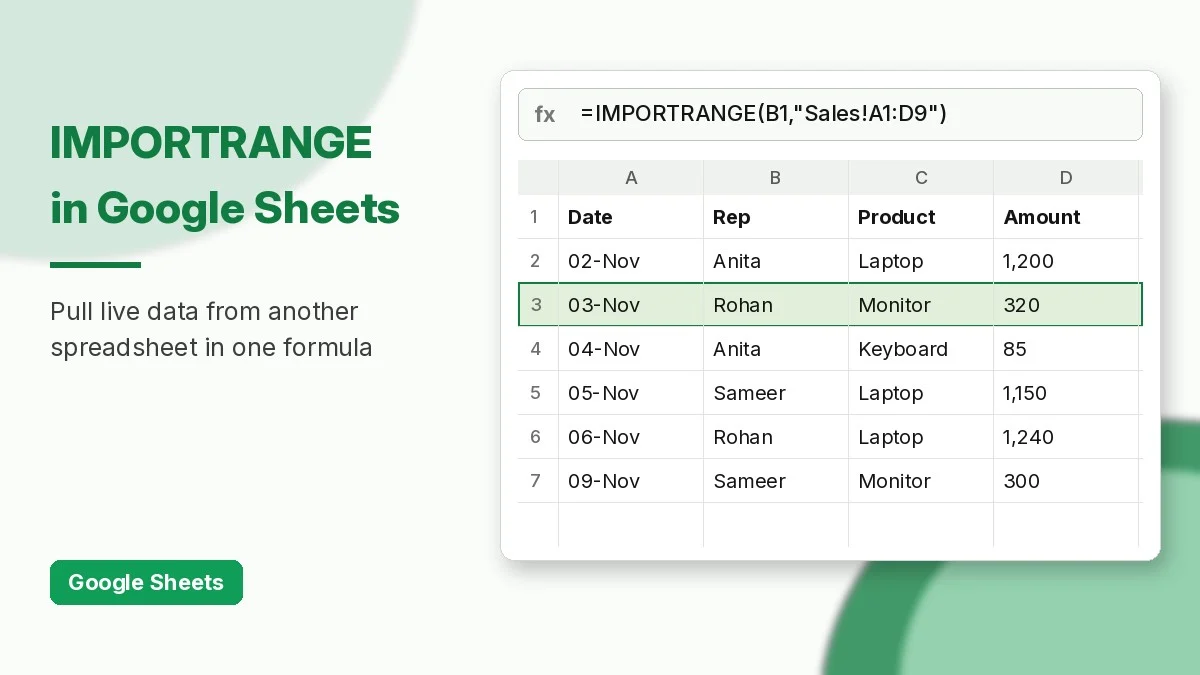
IMPORTRANGE in Google Sheets lets one spreadsheet pull live data from another, so a regional sales file, a budget tracker, or a team roster can feed a single master report without copy-and-paste. When the source changes, the destination updates automatically.
This tutorial covers the syntax, the one-time “Allow access” step, and eight practical formulas, including combining IMPORTRANGE with QUERY, VLOOKUP, and VSTACK. It works the same way in Google Sheets on Windows, Mac, Linux, and ChromeOS browsers, and in the Sheets app on Android and iPhone once access has been granted.
What Does IMPORTRANGE in Google Sheets Do?
IMPORTRANGE copies a range of cells from a source spreadsheet into the cell where you type the formula, spilling the result down and across. The imported values are read-only in the destination: to change them, edit the source file.
IMPORTRANGE Syntax
=IMPORTRANGE(spreadsheet_url, range_string)| Argument | What to enter | Example |
|---|---|---|
| spreadsheet_url | The full URL of the source spreadsheet in quotes, or a cell that contains it | “https://docs.google.com/spreadsheets/d/…” |
| range_string | Sheet name and range as text, or a cell that contains it. Sheet name is optional (defaults to the first sheet) | “Sales!A1:D50” |
The range string can also be a named range or a table reference such as "DeptSales[Sales Amount]", as described in the official Google Docs Editors Help page for IMPORTRANGE.
Sample Data Used in This Guide
The examples assume a source spreadsheet called North Region Sales with a tab named Sales holding this data in A1:D9. In the formulas below, replace the URL with the address of your own source file (copy it from the browser bar).
| Date | Rep | Product | Amount |
|---|---|---|---|
| 2026-11-02 | Anita | Laptop | 1,200 |
| 2026-11-03 | Rohan | Monitor | 320 |
| 2026-11-04 | Anita | Keyboard | 85 |
| 2026-11-05 | Sameer | Laptop | 1,150 |
| 2026-11-06 | Rohan | Laptop | 1,240 |
| 2026-11-09 | Sameer | Monitor | 300 |
| 2026-11-10 | Anita | Monitor | 310 |
| 2026-11-11 | Rohan | Keyboard | 90 |
How to Connect Two Sheets (Allow Access)
- Open the source file and copy its URL from the address bar.
- In the destination file, type
=IMPORTRANGE("paste-url-here","Sales!A1:D9")and press Enter. - The cell shows
#REF!. Hover over it and click Allow access. - The data spills into place. You only need to grant access once per source-destination pair.
If you do not own the source file, you must have at least view access first; otherwise request access from the owner. Once access is granted, any editor of the destination file can import any range from that source.
8 Practical IMPORTRANGE Examples
1. Import a full table
=IMPORTRANGE("https://docs.google.com/spreadsheets/d/SOURCE_ID", "Sales!A1:D9")Returns the headers and all eight rows. Replace SOURCE_ID with the long ID from your own sheet URL.
2. Import an open-ended range that grows
=IMPORTRANGE("https://docs.google.com/spreadsheets/d/SOURCE_ID", "Sales!A:D")Whole-column ranges pick up new rows automatically, but they transfer more data. Keep them to the columns you really need.
3. Use cell references for the URL and range
=IMPORTRANGE(B1, B2)Put the URL in B1 and Sales!A1:D9 in B2. This makes it easy to switch between monthly files without editing the formula.
4. Total the Amount column from another file
=SUM(IMPORTRANGE("https://docs.google.com/spreadsheets/d/SOURCE_ID", "Sales!D2:D9"))Returns 4,695. For very large sources, Google recommends doing the SUM inside the source file and importing just the result.
5. Filter imported data with QUERY
=QUERY(IMPORTRANGE("https://docs.google.com/spreadsheets/d/SOURCE_ID", "Sales!A1:D9"), "select Col2, sum(Col4) where Col3 = 'Laptop' group by Col2", 1)When QUERY reads an IMPORTRANGE result, you must use Col1, Col2… instead of column letters. This returns Laptop sales per rep: Anita 1,200, Rohan 1,240, Sameer 1,150. Learn more QUERY patterns in our Google Sheets QUERY function guide.
6. Look up a value in another spreadsheet
=VLOOKUP("Sameer", IMPORTRANGE("https://docs.google.com/spreadsheets/d/SOURCE_ID", "Sales!B2:D9"), 3, FALSE)Returns 1,150, the first sale for Sameer. XLOOKUP works too: =XLOOKUP("Sameer", IMPORTRANGE(url,"Sales!B2:B9"), IMPORTRANGE(url,"Sales!D2:D9")).
7. Stack data from two regional files
=VSTACK(IMPORTRANGE(north_url, "Sales!A2:D9"), IMPORTRANGE(south_url, "Sales!A2:D20"))Replace north_url and south_url with cell references holding each file’s URL. The older array syntax ={IMPORTRANGE(…);IMPORTRANGE(…)} also works. Both ranges must have the same number of columns.
8. Hide errors while the import loads
=IFERROR(IMPORTRANGE(B1, B2), "Waiting for source data")Use this on dashboards so viewers see a friendly message instead of #REF! while data loads. Remove it while you are setting up, because it also hides the Allow access prompt.
IMPORTRANGE Errors and How to Fix Them
| Error / message | Cause | Fix |
|---|---|---|
| #REF! “You need to connect these sheets” | Access not granted yet | Hover the cell and click Allow access |
| #REF! “You don’t have permission” | You cannot view the source | Request access from the file owner |
| #REF! “Result was not expanded” | Cells below or to the right are not empty | Clear the cells in the spill area |
| #ERROR! “Unable to parse range” | Typo in the sheet name or range string | Check spelling; quote sheet names with spaces: ‘North Sales’!A1:D9 |
| Loading… for a long time | Large range or many import functions | Import smaller ranges or summarise in the source |
Also note that import functions cannot reference cells that depend on NOW, RAND, or RANDBETWEEN, and each request is capped at 10 MB of data. If the source owner turns on “Disable options to download, print, and copy”, new IMPORTRANGE formulas stop working.
Does Excel Have IMPORTRANGE?
No. IMPORTRANGE is a Google Sheets function. In Excel the closest equivalents are external workbook links (for example ='[Sales.xlsx]Sales'!D2) or Power Query via Data > Get Data. LibreOffice Calc uses Sheet > Link to External Data. If you are moving data between apps, our guide on filtering data in Excel and spreadsheets helps once it arrives.
FAQ
How often does IMPORTRANGE refresh?
Changes in the source push to open destination files, and Google also checks for updates about every hour while the file is open.
Can I import from an Excel file in Google Drive?
Not directly. Convert the .xlsx to Google Sheets format (File > Save as Google Sheets) and use the new file’s URL.
Can I edit imported data?
No. Imported cells are read-only. Edit the source, or copy and paste values if you need a static snapshot.
Download the Practice Workbook
The companion workbook below contains the North Region Sales source data, a practice sheet with each task, and a Solutions sheet with every IMPORTRANGE formula as text plus the expected results. Upload the Source sheet to Google Drive to try the formulas live.
Download the practice workbook
The same data as this tutorial, with empty answer cells and a Solutions sheet.
