A PivotTable is a powerful tool to calculate, summarize, and analyze data that lets you see comparisons, patterns, and trends in your data.
Before the start, do have a look on “What’s new in Excel 2019 for Windows“
Table of Contents
Copy the example data in each of the following tables, and paste it in cell A1 of a new Excel worksheet.
| Date | Buyer | Type | Amount |
| 01-Jan | Nikhil | Fuel | $ 7400 |
| 15-Jan | Shammi | Food | $ 6500 |
| 07-Feb | Pardeep | Food | $ 9850 |
| 06-Mar | Shammi | Books | $ 85000 |
| 08-Mar | Tina | Sports | $ 6500 |
| 10-Apr | Tina | Fuel | $ 98600 |
| 15-Apr | Nikhil | Music | $ 800 |
Create a PivotTable to analyze worksheet data
Select the cells you want to create a Pivot-Table from.
Note: Your data shouldn’t have any empty rows or columns. It must have only a single-row heading.
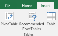
Step 1: Select Insert > PivotTable.
Step 3: Under Choose the data that you want to analyze, select Select a table or range.
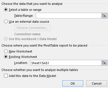
Step 4: In Table/Range, verify the cell range.
Step 5: Under Choose where you want the Pivot-Table report to be placed, then select the New worksheet to place the PivotTable in a new worksheet or Existing worksheet and then select the location you want the PivotTable to appear.
Read Also: Create a Map Chart in Microsoft Excel 2019
Step 6: Select OK.
Building out your PivotTable
Step 1: To add a field to your Pivot-Table, select the field name checkbox in the PivotTable Fields pane.
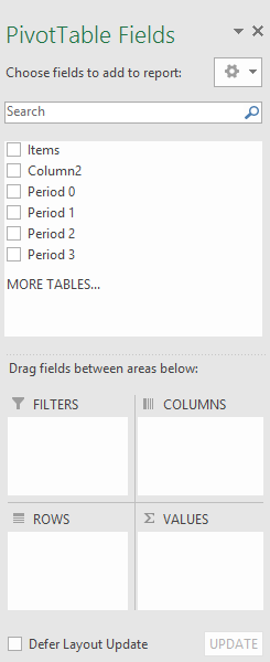
Note: Selected fields are added to their default areas: non-numeric fields are added to Rows, date and time hierarchies are added to Columns, and numeric fields are added to Values.
Step 2: To move a field from one area to another, drag the field to the target area.