Google Sheets QUERY Function: Syntax, Clauses, and Examples

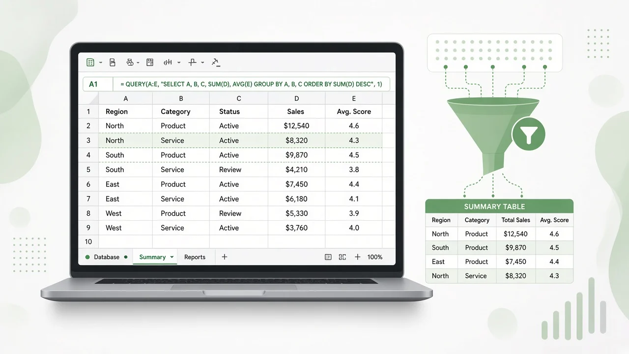
The Google Sheets QUERY function lets you filter, sort, group, and summarize a range with one formula written in a SQL-like language. Instead of chaining FILTER, SORT, and SUMIF, you describe the result you want—”show the region and total sales where status is Closed, sorted highest first”—and Sheets builds the table for you. This guide covers the syntax, every clause in the right order, practical examples, and the mistakes that cause most QUERY errors.

QUERY works the same in Google Sheets on the web, on Windows and Mac browsers, and in the Sheets apps for Android and iOS, so a report you build on a desktop keeps working on your phone.

Google Sheets QUERY Function Syntax

According to Google’s official QUERY documentation, the function takes three arguments:

=QUERY(data, query, [headers])

Argument	Required	What it does
data	Yes	The range to query, for example A1:E500 or an entire sheet range like Sales!A:E. Each column must hold a single data type.
query	Yes	The query text in Google Visualization API Query Language, wrapped in double quotes or supplied from a cell.
headers	No	How many header rows the data contains. If omitted or set to -1, Sheets guesses from the content.

Inside the query string, columns are referenced by their letters (A, B, C) when data is a normal range. When data is an array built with curly braces or another function, refer to columns as Col1, Col2, Col3 instead.

QUERY Clauses and the Order You Must Use

The query language comes from the Google Visualization API Query Language reference. Every clause is optional, but when you use several, they must appear in this order:

Order	Clause	Purpose	Example
1	select	Choose columns or aggregates to return	select A, sum(D)
2	where	Keep rows that match a condition	where C = ‘Closed’
3	group by	Aggregate values across rows	group by A
4	pivot	Turn distinct values into new columns	pivot B
5	order by	Sort the result	order by sum(D) desc
6	limit	Return only the first N rows	limit 10
7	offset	Skip the first N rows	offset 5
8	label	Rename output column headers	label sum(D) ‘Total Sales’
9	format	Apply a number or date pattern	format sum(D) ‘#,##0’
10	options	Set special options	options no_format

Putting order by before group by, for example, returns a parse error even though each clause is valid on its own.

Practical QUERY Examples

The examples below assume a sales log in A1:E with headers in row 1: Date (A), Region (B), Rep (C), Status (D), and Amount (E).

1. Select and filter rows

=QUERY(A1:E, "select A, B, C, E where D = 'Closed'", 1)

This returns the date, region, rep, and amount for every closed deal. Text values go inside single quotes because the whole query already uses double quotes.

2. Total sales by region, sorted

=QUERY(A1:E, "select B, sum(E) where D = 'Closed' group by B order by sum(E) desc label sum(E) 'Total Sales'", 1)

Any column in select that is not aggregated must also appear in group by. The supported aggregation functions are avg(), count(), max(), min(), and sum().

3. Top 5 deals

=QUERY(A1:E, "select C, E where E is not null order by E desc limit 5", 1)

Adding where E is not null keeps blank rows at the bottom of an open-ended range like A1:E out of your results.

4. Filter by a date

=QUERY(A1:E, "select * where A >= date '2026-01-01'", 1)

Dates must use the date 'yyyy-mm-dd' literal. Typing a date like 01/01/2026 directly into the query will not match.

5. Use a cell value as the filter

=QUERY(A1:E, "select B, sum(E) where C = '"&H1&"' group by B", 1)

Here the rep name typed in H1 drives the report. Close the string, join the cell with &, and reopen it—keeping the single quotes around the text value.

6. Pivot regions into columns

=QUERY(A1:E, "select C, sum(E) group by C pivot B", 1)

Each rep becomes a row and each region becomes a column, similar to a PivotTable in Excel, but it recalculates automatically as data changes.

Useful QUERY Comparison Operators

Operator	Meaning	Example
=, !=, <>	Equal / not equal	where D != ‘Lost’
<, >, <=, >=	Numeric or date comparison	where E >= 1000
contains	Text contains a substring	where C contains ‘Shah’
starts with / ends with	Text prefix or suffix	where B starts with ‘North’
like	Wildcards: % (any characters) and _ (one character)	where C like ‘A%’
matches	Regular expression match	where B matches ‘North|South’
is null / is not null	Blank or non-blank cells	where E is not null

Text comparisons are case-sensitive. To match regardless of case, wrap the column in lower(), for example where lower(C) contains 'shah'.

Common Google Sheets QUERY Errors and Fixes

• Mixed data types in a column: QUERY treats each column as one data type, decided by the majority of values. Minority values (for example, a few numbers stored as text) come back as blank. Clean the column so it holds a single type.
• “Unable to parse query string”: usually a clause out of order, a missing single quote around text, or a non-aggregated column missing from group by.
• “No_COLUMN” errors: you used letters (A, B) on an array input. Switch to Col1, Col2.
• Wrong header row: set the third argument explicitly, typically 1, instead of letting Sheets guess.
• Locale separators: in locales that use commas as decimal separators, replace the commas between arguments with semicolons.

QUERY in Excel and LibreOffice Calc

QUERY is specific to Google Sheets. Microsoft Excel 365 and LibreOffice Calc do not have a direct equivalent, so you combine other tools:

Task	Google Sheets	Excel 365	LibreOffice Calc
Filter rows	QUERY … where	FILTER	FILTER (24.8+) or Standard Filter
Group and sum	QUERY … group by	GROUPBY or PivotTable	Pivot Table
Sort results	QUERY … order by	SORT / SORTBY	SORT (24.8+) or Data > Sort
Cross-tab	QUERY … pivot	PIVOTBY or PivotTable	Pivot Table

If you move a workbook from Sheets to Excel, QUERY formulas will not convert, so rebuild them with FILTER and GROUPBY before sharing.

Tips for Faster, Cleaner QUERY Formulas

• Use bounded ranges (A1:E5000) on very large sheets to keep recalculation fast.
• Keep long queries in a helper cell and reference it, for example =QUERY(A1:E, J1, 1), so they are easier to edit.
• Combine QUERY with IMPORTRANGE to report on data stored in another spreadsheet.
• Use label and format so the output is presentation-ready without manual formatting.

FAQ: Google Sheets QUERY Function

Is the QUERY function the same as SQL?

It is similar but not identical. It supports select, where, group by, pivot, order by, limit, and more, but it has no joins and works only on the range you pass in.

Does QUERY work in the Google Sheets mobile app?

Yes. Formulas created on the web calculate in the Android and iOS apps, and you can type or edit QUERY formulas on mobile too.

Why does QUERY return blank cells for some numbers?

The column likely contains mixed data types. QUERY uses the majority type and treats the rest as null, so convert text-numbers to real numbers.

Can QUERY reference another sheet?

Yes. Use a range like Sales!A1:E for another tab, or wrap IMPORTRANGE for another file and refer to columns as Col1, Col2.

Once you are comfortable with the Google Sheets QUERY function, try pairing it with dropdowns from data validation to build interactive dashboards that update automatically.