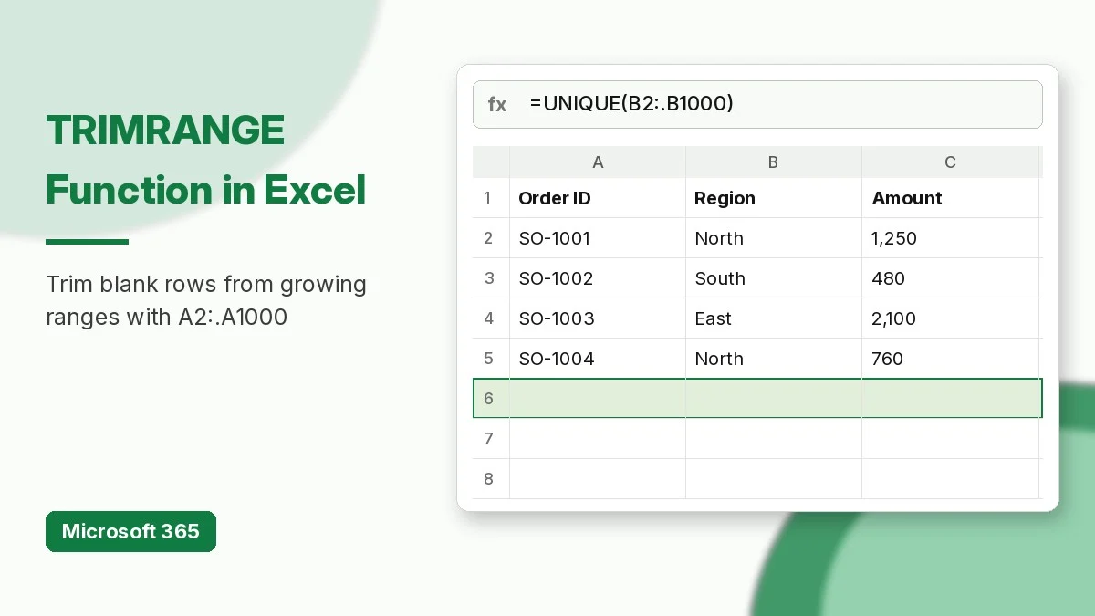
The TRIMRANGE function in Excel removes empty rows and columns from the outer edges of a range, so formulas that point at “room to grow” ranges like A2:A1000 stop returning walls of zeros, blank rows, and bloated spill results. It also comes with a shortcut called trim references (A2:.A1000) that does the same job with a single dot.
In this guide you will learn the syntax, the three trim modes, the trim reference shortcuts, and seven practical examples you can copy into your own workbook. A free practice workbook with the same sample data is linked at the end of the post.
What Is the TRIMRANGE Function in Excel?
Many workbooks use oversized ranges so new rows are picked up automatically. The problem is that dynamic array formulas treat every empty cell in that range as a value. A formula such as =LEN(A2:A1000) spills 999 results, most of them 0, and =UNIQUE(B2:B1000) adds an unwanted 0 to the list.
TRIMRANGE scans in from the edges of the range until it reaches the first non-blank cell and drops everything outside it. Blank cells inside your data are kept; only the leading and trailing edges are trimmed. If you have struggled with oversized spills before, our guide on how to fix the #SPILL! error in Excel pairs well with this function.
TRIMRANGE Syntax and Arguments
=TRIMRANGE(range, [trim_rows], [trim_cols])| Argument | Required? | What it does |
|---|---|---|
| range | Yes | The range or array you want to trim. |
| trim_rows | No | 0 = none, 1 = leading blank rows, 2 = trailing blank rows, 3 = both (default). |
| trim_cols | No | 0 = none, 1 = leading blank columns, 2 = trailing blank columns, 3 = both (default). |
TRIMRANGE is available in Excel for Microsoft 365. It is not included in perpetual versions such as Excel 2024, 2021, or 2019, where the formula returns #NAME?. Microsoft announced the rollout to Windows Current Channel users in the What’s New in Excel (March 2025) update.
Trim References: The Dot Shortcut
Trim references replace the colon in a range with a dotted colon. The dot sits on the side you want trimmed:
| Trim reference | Example | Same as | Trims |
|---|---|---|---|
| Trim trailing (:.) | A2:.A1000 | TRIMRANGE(A2:A1000,2,2) | Blank rows/columns at the end |
| Trim leading (.:) | A2.:A1000 | TRIMRANGE(A2:A1000,1,1) | Blank rows/columns at the start |
| Trim both (.:.) | A2.:.A1000 | TRIMRANGE(A2:A1000,3,3) | Both edges |
Trim references also work with whole columns, so A:.A means “column A, but only down to the last used cell”. The official Microsoft TRIMRANGE documentation lists the same three types.
Sample Data Used in the Examples
All examples use a small order list in A1:C9. Row 1 holds the headers, rows 2-9 hold eight orders, and formulas deliberately point down to row 1000 so that new orders are included automatically.
| Order ID | Region | Amount |
|---|---|---|
| SO-1001 | North | 1,250 |
| SO-1002 | South | 480 |
| SO-1003 | East | 2,100 |
| SO-1004 | North | 760 |
| SO-1005 | West | 1,890 |
| SO-1006 | South | 320 |
| SO-1007 | East | 1,475 |
| SO-1008 | West | 640 |
7 Practical TRIMRANGE Examples
1. Return only the used part of a column
=TRIMRANGE(A2:A1000)The result spills only the eight order IDs (A2:A9) instead of 999 cells. Add an order in row 10 and the spill grows by one row automatically.
2. Count the rows that actually contain data
=ROWS(TRIMRANGE(A2:A1000))This returns 8. Without TRIMRANGE, ROWS(A2:A1000) returns 999 because ROWS counts the size of the range, not its content.
3. Spill text lengths without trailing zeros
=LEN(A2:.A1000)The trim-trailing reference makes LEN spill exactly eight results (each order ID is 7 characters) rather than eight values followed by 991 zeros.
4. Build a clean UNIQUE list of regions
=UNIQUE(B2:.B1000)Returns North, South, East, West. With a normal range the list would end with an extra 0 representing the empty cells.
5. Filter large orders from a growing range
=FILTER(A2:.C1000, C2:.C1000>1000)Both trimmed ranges end on row 9, so they stay the same size and FILTER returns SO-1001, SO-1003, SO-1005, and SO-1007 with their regions and amounts.
6. Sort amounts from a whole-column reference
=SORT(C:.C, , -1)Whole-column references are convenient but slow when they drag in over a million empty cells. C:.C trims at the last used row, so the sorted result is the eight amounts plus the header text at the top (text sorts above numbers in descending order). Use C2:.C1000 if you want numbers only.
7. Trim leading blank rows only
=TRIMRANGE(E1:E20, 1, 0)If a pasted list starts a few rows down (for example, values in E4:E8), mode 1 removes the blank rows above the first value while leaving the bottom of the range untouched. Mode 0 for columns means no column trimming.
TRIMRANGE vs FILTER vs Excel Tables
| Method | Removes edge blanks | Removes blanks inside data | Best for |
|---|---|---|---|
| TRIMRANGE / trim refs | Yes | No | Growing ranges feeding dynamic arrays |
| FILTER(range, range<>””) | Yes | Yes | Lists with gaps in the middle |
| Excel Table (structured refs) | Yes | No | Formatted, structured data sets |
If your data already lives in an Excel Table, structured references resize automatically and you may not need TRIMRANGE at all. For summary reports built on a trimmed range, functions like GROUPBY in Excel accept trim references as their row and value fields.
Common TRIMRANGE Errors and Fixes
- #NAME? – your Excel version does not support TRIMRANGE. Update Microsoft 365 via File > Account > Update Options, or check that you are not on Excel 2024/2021.
- #REF! – the whole range is empty, so there is nothing left after trimming. Wrap the formula in
IFERRORif the range can be empty. - Range is longer than expected – a stray space, apostrophe, or formula returning
""far below your data counts as non-blank. Clear those cells. - Ranges of different sizes – in FILTER or array maths, trim every range the same way so their heights match.
FAQ
Does TRIMRANGE work in Excel 2021 or 2024?
No. TRIMRANGE and trim references are Microsoft 365 features. Older versions show #NAME? when they open a file that uses them.
Does TRIMRANGE remove blank rows in the middle of my data?
No. It only trims the outer edges. Use FILTER to drop interior blanks.
Is A:.A faster than A:A?
In dynamic array formulas, yes, because Excel only calculates down to the last used cell instead of all 1,048,576 rows.
Download the Practice Workbook
Use the companion workbook linked below this article to practise all seven examples on the same order list. It includes an Instructions sheet, a Practice sheet with empty answer cells, and a Solutions sheet with working formulas.
Download the practice workbook
The same data as this tutorial, with empty answer cells and a Solutions sheet.
