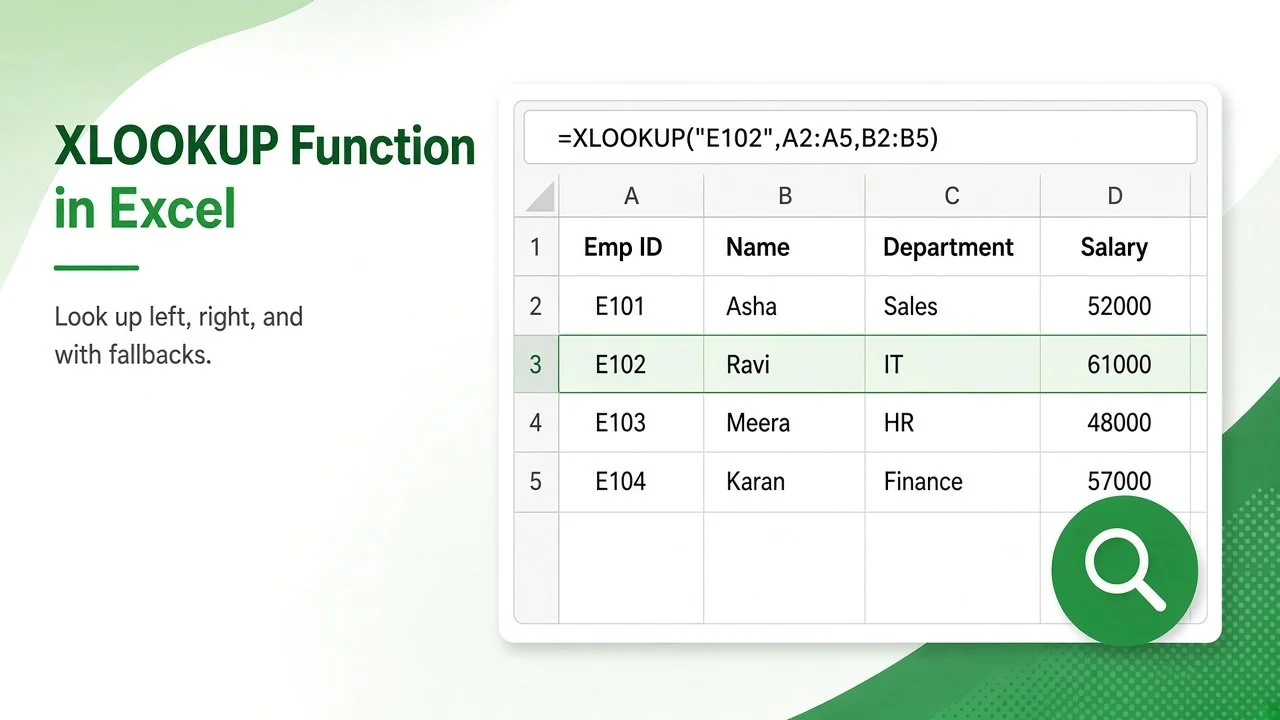
If you still build lookups with VLOOKUP and column index numbers, the XLOOKUP function in Excel will save you time and errors. It searches one range, returns a value from another, looks to the left as easily as to the right, and has a built-in “not found” message. This guide covers the syntax, every argument, and eight practical examples you can copy.
XLOOKUP works in Excel for Microsoft 365 (Windows and Mac), Excel 2021, Excel 2024, Excel for the web, and the Excel apps for iPad, iPhone, and Android. It is not available in Excel 2019 or Excel 2016.
XLOOKUP Function in Excel: Syntax and Arguments
=XLOOKUP(lookup_value, lookup_array, return_array, [if_not_found], [match_mode], [search_mode])| Argument | Required? | What it does |
|---|---|---|
| lookup_value | Yes | The value you want to find |
| lookup_array | Yes | The range or array to search |
| return_array | Yes | The range or array to return a result from |
| if_not_found | No | Text or value returned when no match is found (otherwise #N/A) |
| match_mode | No | 0 = exact (default), -1 = exact or next smaller, 1 = exact or next larger, 2 = wildcard |
| search_mode | No | 1 = first to last (default), -1 = last to first, 2 / -2 = binary search on ascending / descending sorted data |
These argument values come from Microsoft’s official XLOOKUP documentation.
Sample Data Used in This Tutorial
All examples below use this employee list in A1:D7 and a commission tier table in F1:G5 on the same sheet.
| Emp ID (A) | Name (B) | Department (C) | Salary (D) |
|---|---|---|---|
| E101 | Asha | Sales | 52,000 |
| E102 | Ravi | IT | 61,000 |
| E103 | Meera | HR | 48,000 |
| E104 | Karan | Finance | 57,000 |
| E105 | Neha | IT | 66,000 |
| E106 | Vikram | Sales | 50,500 |
| Min Sales (F) | Commission Rate (G) |
|---|---|
| 0 | 2% |
| 50,000 | 4% |
| 100,000 | 6% |
| 200,000 | 8% |
Example 1: Basic Exact-Match Lookup
To return the name for employee ID E102:
=XLOOKUP("E102",A2:A7,B2:B7)Result: Ravi. Unlike VLOOKUP, you do not count columns or add FALSE for an exact match, because exact match is the default. To make it dynamic, type an ID in a cell such as I2 and use =XLOOKUP(I2,A2:A7,B2:B7).
Example 2: Look Up to the Left
VLOOKUP can only return columns to the right of the lookup column. XLOOKUP does not care where the return range sits. To find the ID of an employee by name:
=XLOOKUP("Meera",B2:B7,A2:A7)Result: E103, even though column A is to the left of column B.
Example 3: Return Several Columns at Once
Point return_array at more than one column and XLOOKUP returns the whole row segment:
=XLOOKUP("E104",A2:A7,B2:D7)Result: Karan | Finance | 57000, spilled across three cells. Leave the cells to the right empty, otherwise you will see a #SPILL! error. Our guide on how to fix the #SPILL! error in Excel explains each cause.
Example 4: Show a Friendly Message When Nothing Matches
=XLOOKUP("E110",A2:A7,B2:B7,"Not found")Result: Not found instead of #N/A. This replaces the old IFERROR(VLOOKUP(...),"Not found") pattern, and it only catches missing matches, not other formula mistakes.
Example 5: Approximate Match for Tiers and Brackets
To find the commission rate for sales of 125,000, use match_mode -1 (exact match or next smaller item):
=XLOOKUP(125000,F2:F5,G2:G5,,-1)Result: 6%, because 100,000 is the largest threshold that does not exceed 125,000. A sale of 49,999 returns 2%, and 200,000 returns 8%. With XLOOKUP the tier table does not need to be sorted for match_mode -1 or 1; only the binary search modes (2 and -2) need sorted data.
Example 6: Wildcard Lookup
Set match_mode to 2 to use * (any characters), ? (one character), and ~ (escape):
=XLOOKUP("Ka*",B2:B7,C2:C7,"No match",2)Result: Finance, the department of the first name that starts with “Ka”. Without match_mode 2, XLOOKUP treats the asterisk as a literal character.
Example 7: Find the Last Match
By default XLOOKUP returns the first match from the top. Set search_mode to -1 to search from the bottom up, which is handy for the latest entry in a log:
=XLOOKUP("IT",C2:C7,B2:B7,,0,-1)Result: Neha, the last IT employee in the list. The same formula without the last argument returns Ravi, the first one.
Example 8: Two-Way Lookup With Nested XLOOKUP
An inner XLOOKUP can pick the column by its header, and the outer one picks the row:
=XLOOKUP("E105",A2:A7,XLOOKUP("Salary",A1:D1,A2:D7))Result: 66000. Change “Salary” to “Department” and the same formula returns IT. This replaces INDEX/MATCH/MATCH combinations.
XLOOKUP vs VLOOKUP: Key Differences
| Feature | VLOOKUP | XLOOKUP |
|---|---|---|
| Default match | Approximate (if 4th argument omitted) | Exact |
| Look to the left | No | Yes |
| Inserted columns break it | Yes (column index is fixed) | No (uses ranges) |
| Built-in not-found message | No (needs IFERROR) | Yes |
| Search from the bottom | No | Yes |
| Return multiple columns | One formula per column | One formula, spills |
| Works in Excel 2019 and earlier | Yes | No |
If you are new to lookup formulas, start with our list of 10 essential Excel formulas, then come back to XLOOKUP.
Common XLOOKUP Errors and Fixes
| Error | Likely cause | Fix |
|---|---|---|
| #N/A | No match and no if_not_found value; extra spaces or numbers stored as text | Add if_not_found, wrap the lookup value in TRIM, or convert text-numbers |
| #VALUE! | lookup_array and return_array have different sizes | Make both ranges cover the same rows, e.g. A2:A7 and B2:B7 |
| #NAME? | The Excel version does not support XLOOKUP, or the name is misspelled | Use Excel 2021 or later, or INDEX/MATCH in older versions |
| #SPILL! | A multi-column result is blocked by data | Clear the cells to the right of the formula |
XLOOKUP in Google Sheets and LibreOffice Calc
The same syntax works outside Excel. Google Sheets supports XLOOKUP with the same six arguments, and LibreOffice Calc added XLOOKUP in version 24.8. Workbooks that use it can move between the three apps without rewriting the formulas.
FAQ: XLOOKUP Function in Excel
Is XLOOKUP better than VLOOKUP?
For most new work, yes. It defaults to exact match, can look left, survives inserted columns, and handles missing values. Keep VLOOKUP only when files must open in Excel 2019 or earlier.
Can XLOOKUP return more than one match?
XLOOKUP returns the first (or last) match only. To return every matching row, use the FILTER function, for example =FILTER(B2:B7,C2:C7="IT").
Does XLOOKUP need sorted data?
No. Only search_mode 2 or -2 (binary search) requires sorted data. Exact, approximate, and wildcard matches work on unsorted lists.
Is XLOOKUP case-sensitive?
No. “e102” and “E102” match the same row. For a case-sensitive lookup, combine XLOOKUP with EXACT: =XLOOKUP(TRUE,EXACT(A2:A7,"E102"),B2:B7).
Practice This XLOOKUP Tutorial
Download the companion practice workbook below the article. It contains the same employee and tier data with empty answer cells for all eight examples, plus a Solutions sheet with the working formulas.
Download the practice workbook
The same data as this tutorial, with empty answer cells and a Solutions sheet.
